Artificial Intelligence (AI) in Sports

Dr Patrick Lucey is the Chief Scientist at Stats Perform and has over 20 years of experience working in Artificial Intelligence (AI), in particular face recognition and audio visual speech recognition technology. He also worked at Disney Research (owners of ESPN) where he developed an automatic sports broadcasting system that tracked players in real-time by moving a robotic camera to capture their movements.

Patrick recently talked about the use of Artificial Intelligence in sports, what that means and how we can use AI to help coaches and analysts make better decisions in sport. Artificial Intelligence refers to technology that emulates human tasks, often using machine learning as the method to learn from data how to emulate these tasks. His talk emphasised on the importance of sports data, and provided an overview on the different types of sports data that exist today. Patrick explained what is meant by AI and why is AI needed in sport.

Stats Perform is one of the leaders in data collection in sports, offering a wide range of sports predictions and insights through world-class data and AI solutions. For over 40 years, they have been collecting the world’s deepest sports data, covering over 27,000 live streamed events worldwide with a total of 501,000 matches covered annually from 3,900 competitions. This huge coverage translates into the collection of billions of unique event and tracking data points available in their immense sports databases. To make use of this invaluable dataset, Stats Perform has created an AI Innovation Centre that hired more than 300 developers and 50 data scientists to create a series of AI products with the goal of measuring what was once immeasurable in sport.

Different Types Of Sports Data

Patrick and the Stats Perform AI Innovation Centre have worked on a wide range of different types of data to make predictions on a number of different sports, from football to field hockey, volleyball to swimming using different types of data. There are 3 main types of sports data available: box scores, event data and tracking data. All these types of data facilitate the reconstruction of the story of a match or a particular performance. However, the more granular the temporal and spacial data of a game is, the better the story an analyst can tell.

Box-Score Statistics

The use of high-level box-score statistics (half-time match score, full-time match score, goal scorers, time of goals, yellow cards, etc.) can summarise a 90-minute match of football to provide an idea on how the game was played in just a few seconds. Basic box-score statistics can tell you who won the match, which team took the lead first, when were the goals scored and how close together to each other. Box-score statistics provide a fairly good snapshot of a game and a decent level of match reconstruction.

Box-score statistics Sevilla vs Dortmund (Source: Sky Sports)

Box-score statistics also offer a more detailed level of information. For example, they can illustrate which team had more shots and the quality of those shots by showing the number of shots and shots on goal. They can also explain the distribution of possession between the teams in the match, which team had more corners, committed more fouls, made more saves and so on. Within a few second they can capture the story of the match, which team dominated or how close was that game.

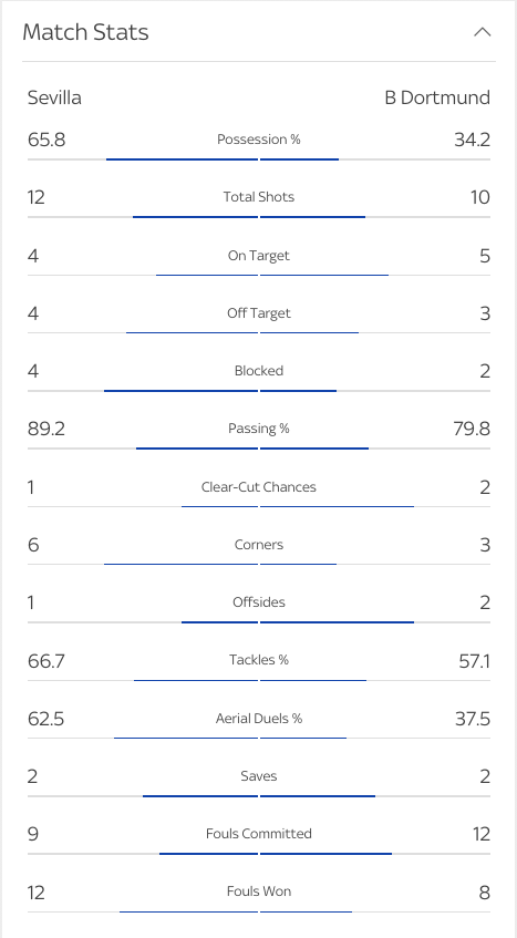
Detailed box-score statistics Sevilla vs Dortmund (Source: Sky Sports)

Event Data

Event data, or play-by-play data, provides a bit more detail than box-score statistics by offering additional contextual information of key moments during a match. For examples, play-by-play commentary of a match can offer textual descriptions of what occurred at every minute of the match. Similarly, spacial data of the game (i.e. spacial location of players) can provide visual reconstructions of some of the key events in a match, such as how a particular goal was scored. While it is not the same as watching the video, it is a quick digitised view of the real-world play that can be reconstructed in seconds.

Text commentary of Sevilla vs Dortmund match (Source: Sky Sports)

Stats Perform, particularly through Opta, is one of the industry leaders in event data collection. They provide event data to sportsbooks through a low latency feed that tells them when a goal, a shot, a dangerous attack or any other key moments occur in close-to-real-time so that the sportbooks can relay that information to their bettors. In these cases, speed of data is crucial, not only to reconstruct a story of what happens on the field through data but to be able to tell that story almost imminently.

Tracking Data

Tracking data is currently the most detailed level of data being captured in sports. It enables the projection of the location of all players and the ball into a diagram of the pitch that best reconstructs a match from the raw video footage of that match. Having a digital representation through tracking data of all players on the entire pitch enables analysts to perform better querying than simply using a video feed that only displays a subsection of the pitch.

Tracking data plotted into a diagram of a football pitch (Source: Patrick Lucey at Stats Perform)

Sources Of Sports Data

Video Footage

The vast majority of data types are collected via video analysis. Video analysis uses raw match footage as the foundation to either manually observe or automatically capture (i.e. computer vision) key events of the match to generate data from. Today, all three types of sports data (box-score, event data and player tracking data) are fundamentally based on video. However, more recently new technologies have been gradually introduced into various sports to collect great details.

Radio Frequency Identification (RFID)

The NFL is now using Radio Frequency Identification (RFID) wearables implemented on players’ shoulder pads to track x and y coordinates of each player’s location on the field.

Radar

In golf, radar and other sensor technology has also been implemented to track the ball’s trajectory and produce amazing visualisations with very accurate detection of the ball.

GPS Wearables

Football and other team sports use GPS devices that, although not as accurate as RFID, can track additional data from the athlete, such as heart rate and level of exertion. These wearable devices have the advantage that they can be used in a training environment as well as a competitive match.

Market Data (Wisdom Of The Crowds)

Market data in sports usually refers to betting data. It is an implicit way of reconstructing the story of the match that relies on people coming up with their predictions where information can be mined from.

AI-Driven Sports Analysis

Sports analysis has traditionally been based on box-score and event data. All the way from Bill James’ 1981 grassroots campaign Project Scoresheet that aimed to create a network of fans to collect and distribute baseball information to Daryl Morey’s integration of advanced statistical analysis in the Houston Rockets in 2007.

However, in the 2010s, tracking data began to set a new path to new ways of analysing sports. Over the last decade, a new era of sports analysis has emerged that maximises the value of traditional box-score and event data by complementing it using deeper tracking data. The AI revolution in sports thanks to tracking data has focused on three key areas:

1. Collecting deeper data using computer vision or wearables

2. Performing a deeper type analysis with that tracking data that humans would not be able to do without AI

3. Performing deeper forecasting to obtain better predictions

Collecting Deeper Sports Data

The main objective of collecting sports data is to reconstruct the story of a match as closely as possible to the one seen by the raw footage that a human or a camera can see. The raw data collected from this footage can then be transformed into a digitised form so that we can read and understand the story of the match and produce some actionable insights.

The reconstruction of a performance with data usually starts by segmenting a game into digestible parts, such as possessions. For each part of this game, we try to understand what happened in that possession (i.e. what was the final outcome of the possession), how it happened (i.e. describing the events that led to the outcome of that possession) and how well it was done (i.e. how well were the events executed).

Currently, the way play-by-play sports data is digitised from the video footage is through the work of video analysts. Humans watch a game and notate the events that take place in the video (or live in the sports venue) as they happen. This play-by-play method of collecting data produces an account of end of possession events that describes what happened on a particular play or possession. However, when it comes to understanding how that play happened or how well it was executed, human notational systems do not produce the best information to accurately reconstruct the story. Humans have cognitive and subjective limitations when capturing very granular level of information manually, such as getting the precise timeframe of each event or providing objective evaluation of how well a play was executed.

In-Venue Tracking Systems

One way tracking data can be collected is through in-venue systems. Stats Perform uses SportVU, which was deployed a decade ago as a computer vision system that installed 6 fixed-cameras on a basketball court to track players at 24 frames per second. Their newer version of SportVU is now widely deployed in football. SportVU 2.0 uses three 4K cameras and a GPU server in-venue to collect and deliver tracking data at the edge in real-time.

Stats Perform SportVU system on a basketball court (Source: Patrick Lucey at Stats Perform)

However, tracking data has a main limitation: coverage. While tracking data provides an immense number of opportunities to do advanced sports analytics, its footprint across most sports is relatively low. This is because for most in-venue solutions a company like Stats Perform requires to be in the venue with all their tracking equipment installed. This is problematic when increasing the coverage of tracking data across multiple events across the world, as it is not realistic to have sophisticated tracking equipment installed in every single pitch, field, court or stadium across the world to cover every single sporting event that takes place every day.

Tracking Data Directly From Broadcast Video

To overcome the limited coverage of in-venue systems, Stats Perform are now focusing their AI efforts in capturing tracking data directly from broadcast video, through an initiative called AutoStats. It leverages the fact that for every sports game being played, there should be at least one video footage of that event being recorded and potentially being broadcasted. The way of getting the best coverage of tracking data is capturing the data directly from broadcasting footage.

PSG attacking play converted to tracking data from broadcast footage (Source: Patrick Lucey at Stats Perform)

This means that the way tracking data is being collected is now evolving away from in-venue solutions to a more widespread approach that uses a broadcast camera. However, the advantage of using in-venue solutions is that you only need to calibrate the camera once. When collecting tracking data off broadcast, you need to calibrate the camera at every frame because it is constantly moving while following the play.

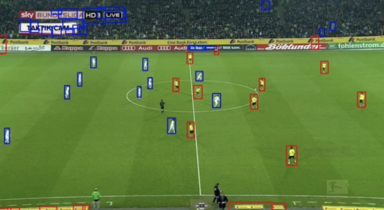
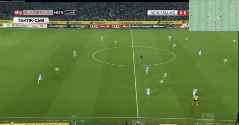
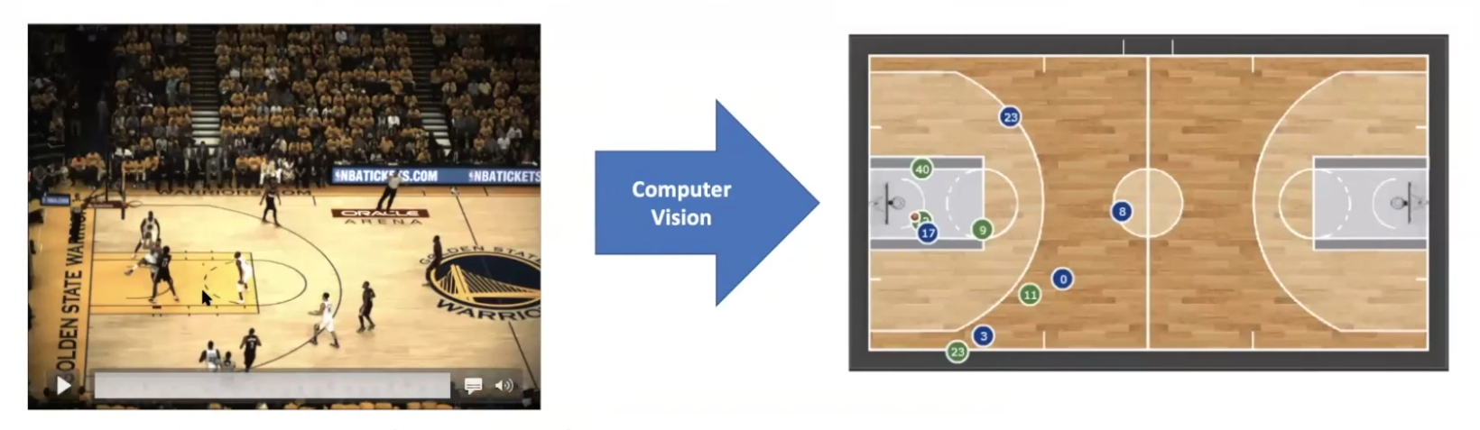
Computer vision systems that collect tracking data directly from broadcasted video footage follow three simple steps:

1. Transform pixels in the video into dots that represent trajectories of the movement of players and the ball. These dots can then be plotted on a diagram of the field for visualisation.

2. The trajectories generated from the movement of the dots over a space of time can then be mapped to semantic events in the sport (i.e. a shot on goal).

3. From the events identified, expected metrics can be derived to explain how well does a player execute on a particular event (i.e. Expected Goals).

Converting Pixels To Dots

Converting video pixels to dots refers the process of taking the video footage of the game and digitally mapping each player movement to trajectories that can be displayed on a diagram of the pitch in the form of dots. The main advantage of this method is the compression of the footage. An uncompress raw snapshot image of a game at 1920x1080px from a single camera angle can be as large as 50MB, which means video footage of that game can be as large as 50MB per frame. If instead of one camera angle you have 6 different camera angles, the data file size multiplies to around 300MB per frame. This is an incredibly high amount of high dimensional data, but not all of it is useful for sports analysis.

Conversion of video footage pixels into dots on a diagram (Source: Patrick Lucey at Stats Perform)

Instead, tracking data representing players on the court or pitch in the form of dots can substantially reduce the size of each frame. For example, in basketball, 10 players, 1 ball and 3 referees can be plotted with their x, y and z coordinates in a digital representation of the court with a size of 232 bytes per frame. This makes tracking data the master compression algorithm on sports video with compression rates of 1 million to 1.

The advantages of using tracking data instead of raw video footage is that it allows to query the dots instead of the pixels in a way that maintains the interpretability and interactivity from the raw video footage. A game can be clearly reconstructed using dots plotted on a diagram of the field to illustrate how each possession happened without the need of the extra detail available in the video footage in the form of millions of pixels.

The way the conversion from pixels to dots occur is via supervised learning, where the computer learns through machine learning processes to map and predict the input data from the pixels to the desired output of the dots. A number of computer vision techniques can be applied to achieve this goal.

Mapping Dots to Events

Once the dots (coordinates) have been generated from the pixel data of the video, the trajectories (movements) of these dots over specific timeframes can be mapped to particular events. For example, in basketball, you can start mapping these dots in the tracking data to particular basketball-related events that describe how certain outcomes occur in terms of tactical themes, such as pick and roll, type of coverages on pick and roll, did the player do a drive or a post up, off-ball screens, hand off, close out, etc. The dot trajectories are mapped to the semantics of a basketball play, and the players involved in that play, using a machine learning model that does that transformation using pre-labelled data.

Mapping Events to Expected Metrics

Expected metrics explain the quality of execution of certain events. The labels assigned to certain events are often not informative enough to explain that event. Instead, expected metrics transform an outcome label of 0 or 1 (goal or no goal) to a probability of 0 to 100% using machine learning. For example, a shot that goes in goal is considered 100% effective. However, a shot attempt that hits the post might be considered 70% effective, even if it did not end up in a goal. Regardless of the final outcome of that event, expected metrics help to evaluate whether an event was more likely to be 0% (unsuccessful), 100% (successful) or somewhere in the middle (ie. 55% successful). This concept of expected metrics is the basis of the Expected Goals (xG) metric in football. Expected Goals can also be extended to passes to calculate the likelihood of a pass reaching a certain teammate on the pitch.

Expected metrics provide an additional degree of context to each situation. For example, in basketball they use Expected Field Goal percentage (EFG) to explain that if a player misses a 3-point shot, rather than simply classify that player as missing a shot we can assess what is the likelihood that an average league player would have scored that shot from a similar situation. This can provide a measure of talent of a player over the league average and better contextualise his performance.

Limitations of Event and Expected Metrics Data

The main limitation of solely using pre-labelled event and expected metrics data using this supervised machine learning process is that not everything can be digitised. Most analysis conducted today are based on events and expected metrics, but these are semantic layers that have been pre-described or pre-categorised by humans. We have put certain patterns of play or combination of player movements into labelled boxes to make it easy to aggregate and analyse sport events. However, the dots generated from tracking data and their identified trajectories open numerous possibilities to perform further analysis that humans can’t do manually by ignoring these pre-labelled categories of patterns of play or specific player movements.

Performing Deeper Sports Analysis

The more granular the data the better analysis we can conduct of a sport. Tracking data provides that necessary level of granularity to conduct advanced analytics. Some of the key tasks that deeper data and better metrics can do much better than humans is strategy, search and simulation.

Strategy Analysis

Marcelo Bielsa once broke down the way he does analysis at Leeds United. His analysis team watches all 51 matches of their upcoming opponent from the current and prior seasons, each game taking 4 hours to analyse. In that analysis, they look for specific information about the team’s starting XI, the tactical system and formations and the strategic decisions that they make on set pieces. However, it can be argued that this methodology is time-consuming, subjective and often inaccurate. This is where technology can come in and help by making the analysis process more efficient than having a team of Performance Analysts spend 200 hours assessing the next opponent.

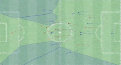
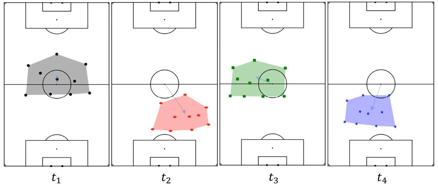
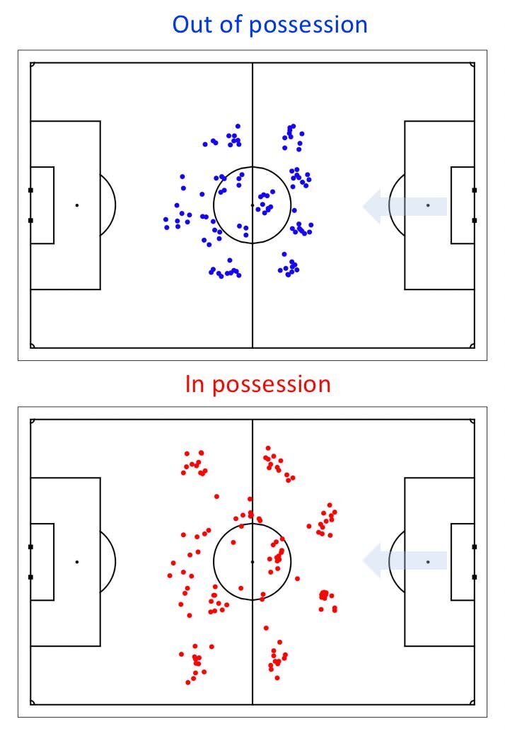
The idea is to transition strategy analysis in sports from a traditional qualitative approach to a more quantitative method. Tracking data has hidden structures. The strategies and formations of a team in a match of football is hidden within all the data points collected from tracking data. Insights on things like formation or team structures do not directly emerge from the tracking data without additional work on the data. This is because tracking data is noisy, for reasons such as that players are constantly switching positions on the pitch. But what tracking data allows you to do is to find that hidden behaviour and structure of a team or players and let it emerge.

Visual representation of a noisy tracking dataset of players in a football pitch (Source: Patrick Lucey at Stats Perform)

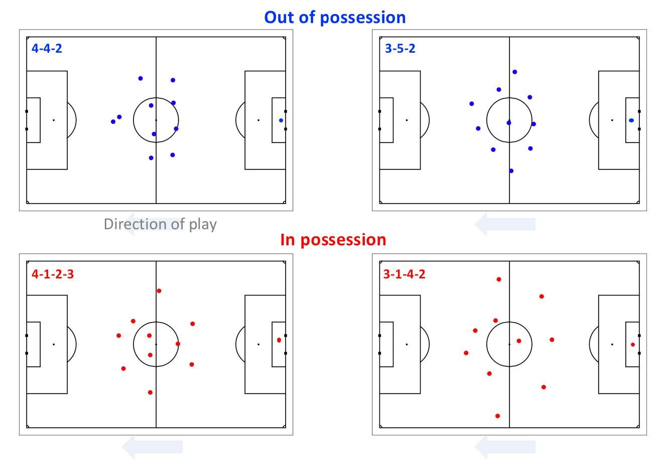
As a way to better visualise and interpret tracking data, Stats Perform have developed the software solution Stats Edge Analysis to enable the querying of infinite formations based on tracking data. The software shows the average formation of players throughout a match, how often each player is in a certain situation, how a team’s structure evolve when they are attacking or defending or how does the formation compare in different context, situations or playing styles.

Formation analysis in Stats Edge Analysis software (Source: Patrick Lucey at Stats Perform)

Search Analysis

How do we find similar plays in sport? How do we search across the history of a sport to find similar situations to the one we are interested in comparing with? One way is to use sport semantics and search using keywords such as a “3pt shot” play in basketball, a “pick and pop” play or a play “on top of the 3pt line”. However, if we want to know where all the players were located in a play, their velocity or their acceleration, as well as all the events that led up to that point, we would need to use too many words to describe that particular play very precisely. In other words, searching across the history of a sport for a similar play using just keywords does not capture the fine-grained location and motions of players and ball and does not provide a ranking of how similar the found plays are to the original play we want to compare them with.

A solution to this problem is to use tracking data. Tracking data is a low dimensional representation of what we see in video. Therefore, instead of using keywords to find a similar play, we could use a snapshot of a play using tracking data as the input in a visual search query. Users could then interact with a visual search query where they describe the type of play they want to search for and the query tool would then output a set of similar plays ranked by the degree of similarity to the play being queried.

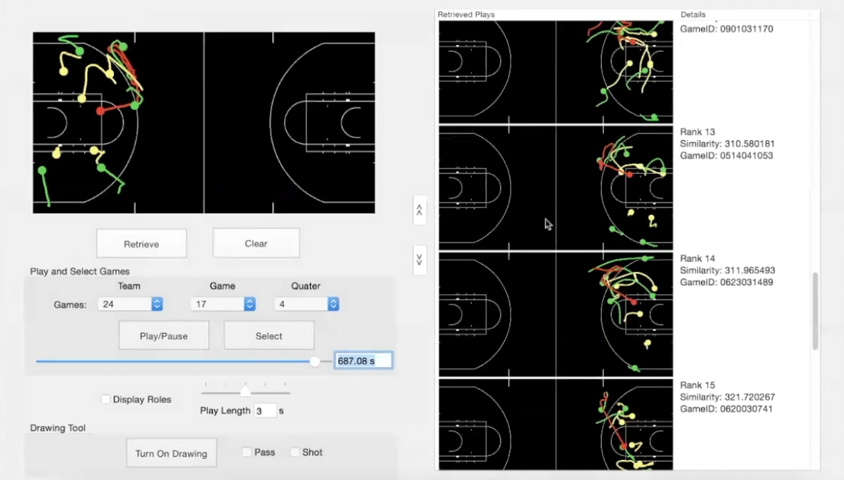
Visual search query of similar plays (Source: Patrick Lucey at Stats Perform)

This type of visual search tool based on tracking data can offer the possibility of drawing out the play to search for. It can also offer the ability to move players around the court and use expected metrics to show the likelihood of a player scoring from various positions. It can even show the changes in scoring likelihood based on the position of the defensive players relative to the player with the ball.

Play Simulation

Technology in sports is entering the sidelines. The type of technology coaches need to evaluate plays during a game and simulate different outcomes needs to be highly interactive. One way Stats Perform has used tracking data to improve play simulations is through ghosting. The idea of ghosting is to show the average play movements at the same time as the live play represented with dots on a diagram of the field. For example, tracking data can display the home team in one colour (blue) and away team in another colour (red), but additionally it can add a third defensive team in a different colour (white) that represents how the average team in the league would defend that same situation.

Ghosting of an average team in the league (white) defending a situation (Source: Patrick Lucey at Stats Perform)

Another way Stats Perform is working with coaches in the sidelines to provide more interactive play simulations is through real-time interactive play sketching. A coach can draw out a play that they want their players to perform on their clipboard and what tracking data and technology can do is to make intelligent clipboards that can simulate how that play drawn by the coach would play out.

Performing Deeper Sports Forecasting

The more granular data available the better we can predict sports performance. Some of the applications of tracking data in forecasting include player recruitment (i.e. which players to buy, trade, draft or offer longer contracts) and match predictions (i.e. accurately predict the final outcome, score and statistics of a match both before the match takes place and in-play).

Player Recruitment

In the NBA, the league has a good level of coverage for tracking data. But what happens when a team wants to recruit someone from college? Tracking data might not exists in college leagues, which forces teams to use a very simplified version of reporting to forecast how that player is going to play once he is recruited onto the team.

This highlights the issue of tracking data coverage. Major leagues have that level of detailed tracking data, but most lower leagues and academy competitions do not. Also, historical matches from major leagues and sports prior to the era of tracking data will not have had the systems and equipment in place at the time to produce highly detailed tracking data. This is where the generation of tracking data through broadcasted video footage can fill that void.

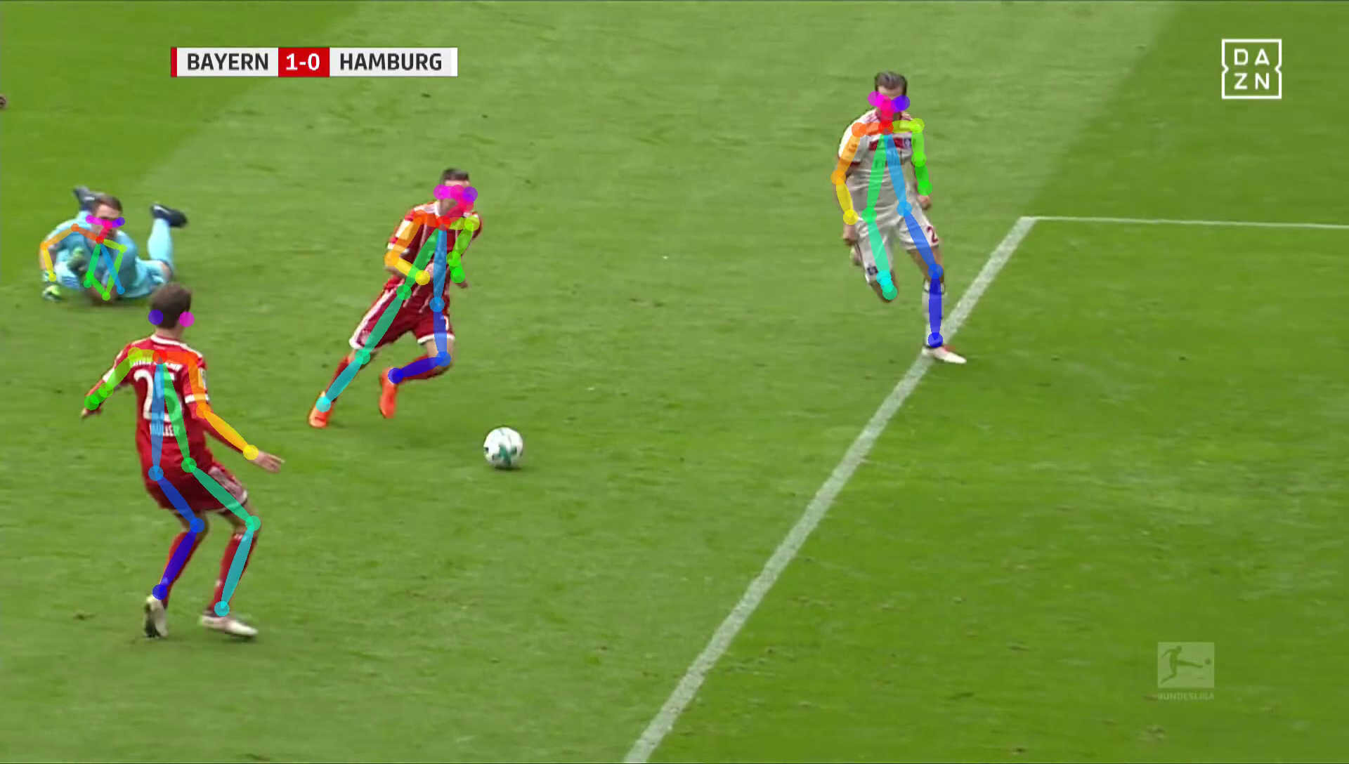
Tracking data using broadcasting footage is the ultimate method to produce detailed recruitment data. Analysts can go back in time and produce data from all the previously untracked players by simply using the footage available from past games. Stats Perform achieves this through AutoStats. AutoStats is a data capture system that can identify where players are located even though the camera is constantly moving by applying continuous camera calibration. It detects body pose of players and can re-identify a player once that player comes back into view after having left the frame. Additionally, AutoStats uses optical character recognition to collect the game and shot clock on every frame, as well as using action recognition to track the duration of player events at a frame-level.

Once that tracking data has been generated from lower leagues or college games, AI-based forecasting can be applied to discover which other professional players is the scouted player of interest most similar to. These solutions can even project a young player’s future career performance. It can use prediction models from historical data of former rookies and their eventual successes to forecast future performances of current prospects.

Given the limited coverage of tracking data in lower and junior leagues, another method to overcome that limitation is to use the already collected event data to maximise the value of the coverage in event data compared to tracking data. Machine learning can define the specific attributes of two players to then compare them with each other. These attributes can be spacial attributes, such as where they normally receive the ball, contextual attributes, such as their team’s playing style (i.e. frequency of counter attacks, high press, crossings, direct plays, build up plays, etc.) and quality attributes, such as expected metrics to capture the value and talent of each player. This method can provide a clear comparison of two different players relative to the context in which they play in. For example, how often is a player involved relative to the playing style of a particular situation.

Taking all this data and the derived attributes from event data, you can then run unsupervised models, such as Gaussian mixture model clustering, to discover groupings of players based on their similarities, and then create a number of unique player clusters that divide pools of players. These clusters can then surface information about the roles that different groups of players play in their teams, whether they are “zone-movers”, “playmakers”, “risk-takers”, “facilitators”, “conductors”, “ball-carriers” or any other clusters that can emerge from applying unsupervised methods. This way, if a team wants to find a player similar to a specific successful player (i.e. players similar to Messi), but with some attributes that are slightly different (i.e. age, league, etc.), they are able to specify that search criteria and find players that fit the profile that they are after.

Match Predictions

There are a couple of ways that AI can help in match predictions. One of them is implicitly through crowd-sourced data. Prediction markets like betting exchange facilitate a marketplace for customers to bet on the outcome of discrete events. It is a crowd-sourced method, and if there are enough participants to represent the entire collective wisdom of the market, with enough diversity of information and independence of decisions in a decentralised way, it is the best predictor you can get. It is an implicit market as we do not know the reason why people have made their betting choices, therefore it is not interpretable. If enough people are participating in these markets, then all possible information to make a prediction is present in that market. If that is the case, it is not possible to beat the accuracy of that market prediction.

Another method is to use an explicit data-driven approach using only data from historical matches together with machine learning techniques to predict probabilities of match outcomes. This method relies on the accuracy and depth of the data available and can only capture the performance present within the data points collected. The advantage of using a data-driven approach is that it can be interactive and interpretable. Also, it only needs the data feed of events, which makes it scalable. However, since not all data might be captured in the dataset used (i.e. injury data), there may be gaps in the analysis that can affect the predictions made.

Sportsbooks normally use a hybrid approach of crowd-sourced data together with data-driven methods to balance the action on both sides of the wager and also to manage their level of risk. They initialise the market with a data-driven approach and human intuition and then iterate based on volume, other sportbooks line and any unique incentive they want to offer to their own customers.

AI-based solutions and tracking data can be used to support these prediction markets, particularly in those markets with insufficient coverage to achieve crowd wisdom. One way of doing so is through the calculation of win probability. Win probability is extensively used across nearly every sport for media purposes. The current limitation of win probability is that it is based on the likelihood that an average team would win given a particular match situation. However, simply using an average may miss contextual information about the specific strengths of particular teams or players involved. The way to overcome that is to use specific models that incorporate the players, teams and line-ups of the match in question.

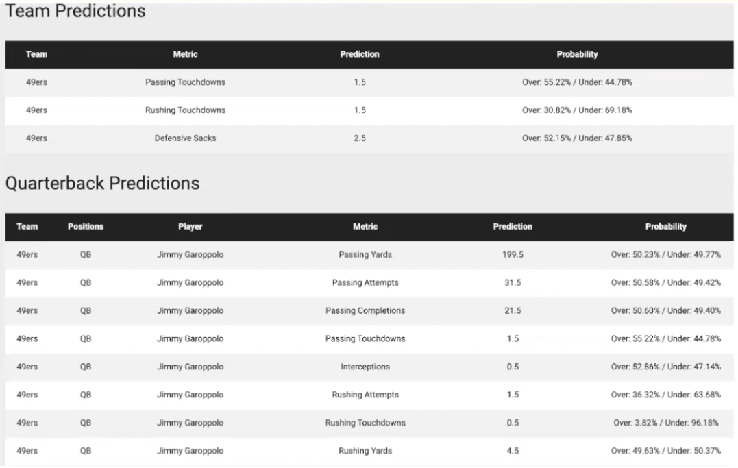
Stats Perform uses models that learn compact representations with features such as the specific opponent, players involved and other raw features describing the lineup to improve prediction performance based on the players involved in the game. This allows them to create specific player props that can predict individual player statistics (i.e. expected points scored in basketball) for each player in the lineup and illustrate that player’s future game performance before the game starts.

Similarly, these predictions can also be made in real-time while a match is being played. For example, using tracking data, in-play predictions in a tennis match can predict who is more likely to win the next point while the rally is taking place. You can even go a level deeper and predict what is the location where the ball will land after the next strike. In football, you could also predict who is the next player who is going to receive a the ball from a pass or where the next shot on goal is going to occur. This is the true value of highly granular levels of data and a data-driven approach to sports analysis.

Automating Data Collection And Match Analysis From Video Footage

Dr Manuel Stein has spent over 7 years researching and analysing player movement using detailed positional football data. His work has focused on the investigation of real-time skeleton extraction to perform match analysis of player movement with the aim of fostering the understanding of comparative and competitive behaviours in football. He has revolutionised the way match and tactical analysis is performed by teaching computers how to measure key playing aspects of the sport, such as team dominance or a player’s control of space derived directly from video footage. Stein has developed an automatic and dynamic model that takes into account the contextual factors that influence the movement and behaviour of players during a match. This novel player detection system automatically is able to display complex and advanced 5-D visualisations that are superimposed on original video footage.

Generating Data From Match Video Footage

The first step for any meaningful quantitative analysis is to obtain highly detailed data to properly test our assumptions. However, gathering highly detailed sport data may be challenging to obtain unless sophisticated tracking technology is used and the results of such tracking are easily accessible to the analyst. On top of that, when it comes to positional player data in football (i.e. xy coordinates of players on the pitch), gaining access to this level of granular data is especially challenging for most analysts. This is the same problem Stein faced during the initial phases of his research and that led him to develop a method for data extraction on his own using television footage and computer vision techniques.

Identifying Players On The Pitch

Stein’s method of extracting data from television footage started with the detection of each player on the pitch. In order to automatically identify the players, Stein addressed the unique colours that are present on the football pitch, more specifically the colours of the players’ shirts. By picking a player in the video, he constructed a colour histogram that best described the most prominent colours in that player’s shirt. Once those colours were identified, he then automatically searched across the video frame for contours of a minimum size that contained those same colours detected from that player’s shirt to spot all other players with the same colour shirt. The computer then automatically calculated the centroid of each detected area (i.e. the players as well as minor noise) and used the average measurements of human proportions to draw boxes enclosing the entire player on the screen.

Colour-based player detection (Source: Manuel Stein at FC Barcelona Sports Tomorrow)

This colour-based player detection method enabled Stein to identify all players on the pitch. The additional noise captured on the sidelines and stadium crowd was later removed by using threshold and ignoring areas that only appear on screen for a brief moment of time. However, this colour-based detection approach has certain limitations depending on the match footage. Lighting variations during matches that kick off under sunlight and finish around dusk do not impact colour perception in humans, but they do so for automatic colour-based player detection systems, as towards the end of the match computers will not be detecting the same colours as they did during kick off.

In order to solve this limitation and develop a system that works on all match conditions, Stein explored additional automated real-time methods to simultaneously extract player body poses and movement data directly from the video footage. One of those methods was the use of OpenPose, a well-known and established computer vision system for human body pose detection. However, OpenPose was not a suitable option when working with football footage, as the system struggles to detect small scaled people on the screen and is also unable to be computed in real-time during a match. Instead, Stein developed and trained his own deep learning model completely from scratch.

Body pose detection system (Source: Manuel Stein at FC Barcelona Sports Tomorrow)

Stein’s human body detection model uses a skeleton model based on a hierarchical graph structure that represents a body’s pose. Every node on the hierarchical graph corresponds to the position of a body part from the person’s skeleton such as joints, ears, eyes and so on, called key points. The edges of this hierarchical graph represent an anatomical correct connection between two body parts. Stein’s body pose detection process followed two stages: the detection of individual body parts followed by the probabilistic reconstruction of the skeletons by connecting all identified body parts together. The constructed skeletons of the players were then overlayed on the original video footage for easy visualisation. Stein model’s estimation accuracy results outperformed those of OpenPose when estimating the skeletons on medium-scale people from the Microsoft COCO dataset. Moreover, their model architecture is also optimised for real-time and low latency video analysis, unlike OpenPose which struggles to run on resolutions of close to 4k.

Identifying The Ball

The next step was to detect the ball. For that, the model followed a two-step approach: a per-frame candidate detection step followed by a temporal integration phase. It first detected all possible objects on the screen that could potentially be the ball by using a convolutional neural network. The computer detected things such as the penalty spot, the corner kick spot, the centre spot, white football boots or the ball itself as being possible candidates. The next step was to identify an accurate and realistic ball trajectory over a period of time from the previously identified candidates using a recurrent neural network. This enabled the model to specify which one out of the previously detected objects was indeed the ball, as it was moving throughout the footage as a ball would be expected to move. By using this approach, the ball could be tracked even when it was not visible on the video footage. For instance, the computer continued to track the ball even when a player picked it up before a penalty kick and happened to hide it from the camera.

Determining Player And Ball Location On The Pitch

Once both players and the ball have been detected, the following step is to determine their location on the full football pitch. The challenging part in this section is the fact that the camera is continuously focusing on different parts of the pitch rather than the pitch as a whole. To solve this issue, Stein had to produce a static camera shot by creating a panoramic view of the complete stadium using a subset of input frames from the video footage (i.e. all frames from the first two minutes of a match). The overlap of all these snapshots from the video footage was then used to recreate a panoramic view of the pitch that allowed Stein to calculate the pitch’s homography. He was then able to identify how two different images connected together, or detect whether one image was simply a subset of a larger image. The homography calculation then enabled Stein to project each of the frames from the video footage into the panoramic view of the pitch as a unique reference frame and fully visualise where on the full pitch each frame took place.

Projection of frames on the panoramic view of the full pitch (Source: Manuel Stein at FC Barcelona Sports Tomorrow)

With all players and the ball correctly identified and their position accurately projected on a panoramic view, the next step was to project these player locations into a normalised football pitch to start generating usable positional data for further analysis. By providing the system with a standard image of a football pitch, a user can select a minimum of four points both from the panoramic view and their image of the pitch in order for the system to use the homography calculations from the panoramic view and translate them into the standard image of the pitch. This allows the system to automatically plot accurate player positional data on a standard diagram of a football pitch.

Player locations and movements illustrated in real-time on a diagram of the pitch on the top right corner (Source: Manuel Stein at FC Barcelona Sports Tomorrow)

Automatically Measuring Contextual Information From Video

Stein took his research further by incorporating the tracking of elements in a match that are not clearly visible to a computer, areas such as the dependencies, influences and interactions between players during the various scenarios of a game. For a fully automated football analysis system to work, this context information that is obvious to humans also needs to be taken into account and measured by the computer. In a dynamic team sport like football, players are more than simple and independently moving dots on a pitch. There is a complex network of interactions and dependencies that dictate how a player reacts to a situation, how they cooperate with teammates and how they attempt to prevent the opposing players’ actions.

Interaction Spaces

One way to automatically measure contextual information from player positional data was to identify the specific regions on the pitch that are controlled by the different players. Stein argued that each player has a surrounding area around them that he fully controls based on his position on the pitch. These control regions are what he called ‘interaction spaces’ on the pitch that a player can reach before any opposing player or the ball could reach that same space. The size and shape of these interaction spaces are influenced by player speeds and directions, as well as the distance between the players and the ball. This is because players further away from the ball may have more time to react.

Interaction spaces for each player (Source: Manuel Stein at FC Barcelona Sports Tomorrow)

On top of that, competition between two opposing players to control a certain zone has also an impact on the shape of these interaction spaces, as players from the opposing team will aim to restrict certain opposing player movements. Therefore, when defining interaction spaces on the football pitch, Stein aimed to consider these interdependencies that may restrict a player from reaching a particular zone before an opposing player to maintain ball possession. This can be seen in the above illustration between the blue team’s defensive line and the red team’s forwards, where players that are close to opposing players may restrict each other’s interaction spaces. Lastly, Stein was able to leverage the pitch visualisations of the previously recorded positional data and enrich it with additional context information that clearly illustrates each interaction space in real-time.

Free Spaces

An alternative way of contextualising automatic tracking data was the inclusion of free spaces. Stein calculated free spaces by segmenting the pitch into grid cells of 1 squared metre. He then assigned each respective cell to the player with the highest probability of reaching that cell in relation to the distance to the cell, their speed and direction of movement. Similarly to interaction spaces, free spaces where the cells from the grid that a player could reach before any other opposing player. Ultimately, free spaces represented the pitch regions a specific team or player owned.

All free spaces identified for a team in blue (Source: Manuel Stein at FC Barcelona Sports Tomorrow)

To evaluate which free zones were more meaningful for analysing, Stein ranked all free spaces on the pitch by their value in relation to their respective sizes, number of opposing players overlapping such spaces and the distance to the opposing goal.

All high value free spaces shortlisted for a team in blue (Source: Manuel Stein at FC Barcelona Sports Tomorrow)

Dominant Regions

Stein expanded his concepts of region control on a football pitch by using similar calculations to those of interaction spaces to create a model that highlights the dominant regions for each team. These dominant regions are calculated by looking at areas on the pitch that can be reached by at least 3 players of the same team simultaneously. Ultimately, they represent the areas in which a particular team has substantially more control over the other.

Dominant zones by players in the blue team (Source: Manuel Stein at FC Barcelona Sports Tomorrow)

Cover Shadows

Similarly, Stein extended the concept of interaction spaces to calculate player cover shadows, referring to the area a player can cover in relation to the position of the ball. In other words, a player has full control to prevent a ball from reaching their cover shadow region. Cover shadows can be thought of as a hypothetical light source coming from the ball at a 360 degree angle. These cover shadows represent the regions that the player is able to control before the ball gets to them.

Cover shadows illustrating a player’s area coverage in relation to the ball (Source: Manuel Stein at FC Barcelona Sports Tomorrow)

Applications Of This Automated Player Tracking System

When looking at the possible applications of his automated tracking system, Stein had to consider the roles of Performance Analysts and the coaches. For a Performance Analyst, video and movement data are key when analysing the strengths and weaknesses of their team and the opposition. On one side, analysts have a window on their screens with their video analysis software opened, such as SportsCode or Dartfish, to notate events and analyse playing actions. While on the other side, they have another window with the original video footage of the match that they use to verify and interpret any observations captured from their coding. Often what this means is that the analyst is looking at two different windows and comparing them to one another. While this is common practice in the field of Performance Analysis, the exercise of switching focus between two screens may often prove to be an inefficient approach to video analysis. Focusing on two windows simultaneously can prove significantly challenging to the human eye, often leading to a ‘pause and play’ exercise during analysis.

Stein aimed to solve this problem by combining the benefits of the visualisation of the pitch from his new automatic player tracking system with the original match footage. By simply inverting the homography from the abstract pitch into the video footage, he was able to draw visualisations directly on the real pitch. This allowed him to illustrate in real-time different types of analysis, from evaluating offensive free spaces to looking at players’ interaction spaces.

Interaction spaces automatically displayed directly on real match footage (Source: Manuel Stein at FC Barcelona Sports Tomorrow)

Stein’s dynamic and automatic real-time visualisation offered a whole new range of design opportunities for match analysis in football. For instance, the system was able to change a player’s shirt colour based on their behaviour (i.e. based on fatigue). It was also able to illustrate the best passing options available to the player with the ball.

Automatically computed best passing options (Source: Manuel Stein at FC Barcelona Sports Tomorrow)

This novel tracking method provides an invaluable automatic measurement of the context of a match situation. However, similar to any other analytical tools, it needs to be correctly applied in order to make a difference to team and player performance. Aside from the clear operational efficiencies brought by the automation of tedious notational work, the benefits in knowledge acquired from this system needs to be appropriately incorporated into the analysis loop. For instance, data on free spaces can be used to automatically detect suboptimal movements from players and suggest potential improvements for such behaviours. For example, an analysts can select specific situations where there was a shot on goal or dangerous play by the opposition to then identify which of their own players had control over free spaces that could have prevented such occasion. Once a selection of possible players have been identified, analysts can assess which one of those players lost control of their space the fastest and how such player could have kept control over his opponent. The identified player can then receive information about which should have been his optimal position on the pitch and their control of field space in order to reduce the free spaces towards his own goal left to be exploited by their opponents. Stein’s system is able to provide this guidance to analysts, coaches and players by automatically calculating the player’s moving trajectory based on his speed and interactions space and suggest an optimal realistic movement for that player, from the starting position to the optimal point. This means that the system can automatically suggest improvements in collective behaviour based entirely on the contextual information being processed.

Click and drag interactivity (Source: Manuel Stein at FC Barcelona Sports Tomorrow)

The system also offers interactivity, where analysts and coaches can drag and drop players around the pitch to explore the different control spaces the player would benefit from if they were in a different location of the pitch. By moving a player to a different location, the system automatically updates the player’s trajectory and interaction spaces relating to their new location and the other players around him. This gives coaches and analyst the possibility to interact with the analysis and to adapt the system based on their own acquired knowledge of the sport.

Automated systems such as the one developed by Manuel Stein are bringing exciting levels of innovation to the sport by directly integrating data and video together. Thanks to these systems, football experts, coaches and analysts become more aware of the power of analytics once they are shown the context of real world scenarios, which in turn leads to better analytical approaches being developed that are better incorporated into the daily realities of the roles of analysts and coaches. Ultimately, it reduces or completely removes numerous tedious and time consuming work performed by analysts today in a revolutionary way that frees up time away from simple data collection which can in turn be placed in more dedicated and advanced analysis of the sport.

Further Reading:

• Manuel Stein’s publications

• Stein, M., Janetzko, H., Breitkreutz, T., Seebacher, D., Schreck, T., Grossniklaus, M., Couzin, I. & Keim, D. A. (2016). Director's cut: Analysis and annotation of soccer matches. IEEE computer graphics and applications, 36(5), 50-60. Link to article

How The NFL Developed Expected Rushing Yards With The Big Data Bowl

Michael Lopez, the Director of Data and Analytics at the NFL, recently discussed at the FC Barcelona Sports Tomorrow conference the way that his Football Operations team and the wider NFL analytics teams leverage a large community of NFL data enthusiasts to obtain a better understanding of the game of American Football. In his talk, Michael walked through the journey that the NFL took to develop expected rushing yards, a concept that began as an initial idea within their Football Operations group and ended up making its way up to the NFL’s Next Gen Stats Group and the media.

What To Analyse With The Data Available In The NFL?

The first step that the NFL Football Operations team took to figure out what should be answered with the use of data is to try to understand what the general public thinks about when they watch an NFL game. To figure this out, they looked at a single example of a running play in a 2017 season game between Dallas and Kansas where the running back, Ezekiel ‘Zeke’ Elliot took 11 yards from a 3rd down and 1 yard-to-go. This run by Zeke Elliot eventually allowed Dallas to successfully move further down the field and score points.

Statisticians at the NFL then tried to understand what can be learned from a play like this one by breaking down the play to obtain as many insights on the teams involved, the offence, the defence, and even the ball carrier. An initial eye test by simply looking at the video footage told the analysts that in this particular play Zeke Elliot - the ball carrier - had a significant amount of space in front of him to pick up those 11 yards. But how could data be applied to this play to tell a similar story? To do so, NFL analysts first needed to take a look at the data and information that was being collected from that play, to understand what was available to them and the structure of the datasets that will allow them to come up with possible uses for that data.

There are three types of data being collected and used by the NFL analytics teams: play level data, event level data and tracking level data. Each one of these types of data present different levels of complexity, with some having been around for longer than others.

• Play Data:  

  This data contains the largest amounts of historical records and includes variables like the down, distance, yard line, time on the clock, participating teams, number of time outs and more. It also includes some outcome variables like number of yards gained, passer rating to evaluate QBs, win probability and expected points. 

• Event Data:

  This data is generated from notating video footage. It is usually performed by organisations such as Pro Football Focus or Sports Info Solutions by leveraging their football expertise. These companies tag events using video analysis software and collect data points such as the offensive formation, number of defenders in the box, defenders closer to the line of scrimmage, whether a cover scheme was man versus zone, the run play called and so on.

• Tracking Data:

  This type of data refers to 2-D player location data that provides the xy coordinates as well as the speed and direction of players. It is usually captured at 10fps using radio frequency identification (RFID) chips located on each player’s shoulder pads as well as the ball. It tracks every player during every play of every game. This is the most novel type of data being collected by the NFL. Player tracking data was only started to be shared with teams from the 2016 season onwards.

2D Player Tracking Data (Source: Mike Lopez at FC Barcelona Sports Tomorrow)

The sample sizes of data that is available for NFL analysts to come up with new metrics varies for each one of these data types. When it comes to play data, there is an average of 155 plays per game, and 256 games played in a single season. This means that for the longest time in the sport, analysts have had a maximum of almost 40,000 plays per season to figure out the answers to NFL analytics questions. A similar scenario is true with event data, where the dataset available to NFL analysts will be a multiple of the number of observations you are producing through the notation of events from a maximum of 40,000 plays per season.

A very different scenario occurs with player tracking data, where the sample size is substantially larger. With 2-D player location of each player being tracked at 10fps on plays that usually last 7 seconds, the data collected jumped from those 155 observations (plays) per game in play-level data to between 200,000 and 300,000 observations for a single game for tracking-level data. This brought a more complex dataset to the sport and opened the door to new questions and metrics to be explored by NFL analysts.

Applying The Available Data To The Analysis Of The Game

There are various approaches that the NFL analyst could have taken to evaluate the running play by Dallas where Zeke Elliot gained 11 yards. Ultimately, they wanted to figure out what was the likelihood of Zeke Elliot picking up those 11 yards in that running play.

One of these approaches was to assign a value to the play to evaluate how the running back performed by using metrics like yards taken, win probability or expected points. By using this play level data, analysts would be merely calculating the probability of those 11 yards being achieved using simple descriptive metrics, such as the fact that it was a 3rd down and 1 yard-to-go in a certain location of the field during the first minutes of a scoreless match. If they then compared Zeke Elliot’s outcomes based on similar plays, all of these metrics would have shown positive values, as gaining yards would have had an increase in both the team’s win probability and expected points. Zeke Elliot’s 11 yard run may have well been above average when you describe plays using play level data. However, this approach would be missing the amount of credit that the running back, the offensive line and the offensive team should really receive from this outcome given the specific situation they faced.

Another approach was to leverage event level data to provide additional context of the play. This type of data could have helped understand Zeke Elliot’s performance by providing additional variables, such as the number of defenders in the box or the play options available, which would have allowed to compare the probability of taking 11 yards against other plays with similar characteristics. However, these approach may have also shown positive results due to the relative large yardage gain Zeke Elliot achieved for the run. Moreover, appropriately describing the situation only using event data may be challenging or inaccurate as it is conditioned to the video analyst’s level of football expertise and ability to define the different key elements of the play.

Instead, NFL analysts decided to make use of the 2D player tracking data for that play to come up with the spatial mapping on the field. By having a spatial mapping of the field, analysts could visualise the direction and speed in which each player was moving during the duration of the run, as well as what percentage of space on the field was owned by different players of each team. This gave analysts an idea of the areas that were owned by the offence and the ones owned by the defence, providing them with better understanding of the amount of space in front of the running back, Zeke Elliot, to take on extra yardage. The information obtained from the spatial mapping could then be used to calculate yardage probabilities given the extra condition of space to more accurately assess how well the offensive team performed.

Spatial Mapping of Zeke Elliot’s Run (Source: Mike Lopez at FC Barcelona Sports Tomorrow)

In this diagram above, it is clear that the offense owned most of the space in front of Zeke Elliot, not only 11 yards ahead but even 15 yards in front of the running back, with defenders nowhere close to him. As oppose to evaluating the play with play or event level data, using tracking data raised further questions on the performance of Zeke Elliot on that play, as it may not be as positive as the other approaches may have suggested given the amount of space he had in front of him.

Following this example, NFL analysts next tried to answer the question of how to leverage player tracking data more widely to better understand what happens during plays. The NFL Football Operations analysis team wanted to learn more about how this data could be used to compare the performance of players given the positioning, direction and speed of all 23 players on the field. More specifically, it involved understanding the probability distribution of all possible yardage increments - i.e. the running back taking or losing 5, 10, 15, 20 yards and so on – to obtain a range of outcomes with their likelihoods that would then allow analysts to compare different performances in different plays. A probability distribution that is based on yardage increments could then be explored further to provide analysts additional insights on first down probability, touchdown probability or even probability of losing yardage on a given play in spatial mapping terms. Ultimately, this probability distribution could be turned into an expected yards metrics for running backs by multiplying each yard by the probability of reaching that yardage and summing up all the values together.

Leveraging AWS And The Wider NFL Community

The main goal of the NFL Football Operations team was to better understand player and team performance by leveraging the new xy spatial data from player tracking to come up with new metrics, such as expected yards, touchdown probability or run play. The NFL Football Operations team worked closely with the NFL’s Next Gen Stats Group to understand the value that such metric will provide to the sport and define a roadmap of how to go about developing such metrics. Sunday Night Football and other media broadcasters also showed a strong interest in using this new metrics to better evaluate performances on air.

In their first attempt at producing new metrics from player tracking data, NFL analysts partnered with data scientists from Amazon Web Services (AWS) to figure out how this large dataset of player tracking data could be used to come up with new football metrics. Unfortunately, after trying a wide set of tools, ranging from traditional statistical methods to gradient boosting and other machine learning techniques, the NFL Football Operations and AWS partnership never produced results that were satisfactory enough to be used by NFL Next Gen Stats Group or the media. While they learned about possible application of the spatial ownership distribution on the field, when it came down to validating the results against the one example of Zeke Elliot’s 11 yard running play, the results did not provide enough confidence to be used for the wider analysis of the sport. The AWS-NFL data science collaboration had reached a dead-end in their analysis.

Source: NFL Next Gen Stats

In order to unblock this situation and produce a metric from tracking data that would match what was seen in the video footage, the NFL Football Operations team leveraged the crowd sourcing wisdom in football statistics through the Big Data Bowl, an event they organise since 2019 and that was also sponsored by AWS. The Big Data Bowl is an annual event that serves as a pipeline for NFL club hiring, as it helps identify qualified talent that can support the NFL’s Next Gen Stats domain in analysing player tracking data. Since player tracking data has not been around for a long time, this event enabled the NFL to understand what the right questions to ask from this data are and how to go about answering them. The Big Data Bowl also serves core NFL data analytics enthusiasts who want extra information on the sport by helping them understand more about the NFL through more intuitive metrics that more clearly reflect how fans think about the game. For the past couple of years, this event has also proven to be a great opportunity for NFL innovation, as it has successfully tapped into the global data science talent to solve problems that a team of data scientists at AWS and the NFL could not resolve on their own. The first Big Data Bowl in 2019 saw 1,800 people sign up to take part, with 100 final submissions from having completed the task given. Out of these pool of analysts and data scientists, 11 went on to be hired by NFL teams and vendors. The winner of the 2019 competition is now an analyst for the Cleveland Browns.

Source: NFL Football Operations

The success of the Big Data Bowl 2019 edition meant that the NFL Football Operations would decide to take advantage of the Big Data Bowl 2020 event to develop their highly anticipated expected yards metric from the 2D player tracking data. Instead of trying to figure out the metric internally on their own, they took a ‘the more the merrier’ approach to exploit the opportunities available from the analytics talent across the world. The NFL Football Operations team shared the exact player tracking data with the participants in the event, who were given the task of predicting where the running back would be after a handoff play, such as the one earlier discussed between Dallas and Kansas. By receiving this player tracking data, participants now had valuable data points specifying the positions of all the players on the field, their speed, the number of players in front of the running back, who those players were, and more. All they needed to do is to come up with a method that would allow the NFL to understand whether Zeke Elliot’s performance was above or below average.

The competition launched in October 2019, when data was shared and released by the NFL. There were a total of 2,190 submissions for the event, with participants from over 32 countries. The launch was followed by a 3-month model building phase to allow teams to develop their algorithms. These algorithms were later evaluated in real time during the 5-week model evaluation phase of the competition. This model evaluation phase tested each algorithm’s predictions using out-of-sample data and compared the results with the true outcomes. The competition used Kaggle as their main data science platform to encourage interactions and communication across teams through forums. It also provided a live leaderboard where teams could see how well their algorithms were performing against other teams. Team scores were completely automated based on how accurate the algorithms were against real data. The winning team was a team called ‘The Zoo’, formed by two Austrian data scientists, who came up with a 5 dimensional convolutional neural network containing only five inputs: the location of the defenders, the routed distance between defenders and the ball carrier, the routed speed of the defenders and ball carrier, the routed distance between all offensive players and all defensive players, and the routed speed of all offensive players and all defensive players. They eventually presented their model in the NFL Scouting Combine event that was attended by more than 225 teams and club officials. They also received a cash prize of $75,000.

The winning team’s model results significantly outperformed those of the rest of participants. The calibration of their model showed an almost perfectly calibrated model where their predicted number of yards closely matched the observed number of yards from an out of sample dataset. Their model was able to take data from a carry and predict the yardage that carry would achieve, not only for small gains of 3 to 5 yards but also for longer yard gains of 15 to 20 yards, which are rarer in the sport. Thanks to their model, an expected yards metric could be produced for every running play. This now provides a valuable tools to assess performance of running plays such as the one by Zeke Elliot. For example, when a player takes 29 yards from a run, if the model calculated an expected yardage gain of 25 yards for that run given the spacing the running back had at the handoff, that player should only get credited for having achieved 4 yards above the average. This new way for interpreting a 29 yards run would not have been possible unless a model successfully conditioned its probability calculation based on the space available to the running back to determine whether that player has performed above or below expectation.

Winning team’s calibration plot (Source: NFL Football Operations)

The benefits of the Big Data Bowl format was that unlike hackathons, where participants may only get one or two weekends to produce something of value, this type of event enabled enough time for the teams to navigate the complex player tracking data set and come up with actionable insights. The NFL was then able to immediately obtain and share the new derive metrics with the media and their Next Gen Stats group to be used for their football analytics initiatives. Thanks to this approach, clubs can now better evaluate their running backs. Moreover, other industries, such as the growing betting industry in the USA may also benefit from the development of expected yards for their betting algorithms. Lastly, expected yards are now being widely used by NFL broadcaster to show whether running backs are performing well or not during the duration of a game. Metrics like this one would not have been possible without the NFL tapping to a global talent pool of data scientist to help them come up with this novel expected yards metric.

The NFL is continuing to run their Big Data Bowl this year, with their 2021 edition being a lot more open ended than previous editions. This time the task focuses on defensive play. They are sharing pass plays from the 2018 season and are asking participants to come up with a model that defines who are the best players in man coverage, zone coverage, how can the model identify whether the defence is man or zone, how to predict whether a defender will get a penalty and what types of skills are required to be a good defensive player. It leaves the interpretation and approach to the participants to define and allows them apply the right conditioning to the data provided. This approach of opening your data to the public in order to push data innovation forward has proven successful and would be interesting to see if other sports will adopt similar initiatives.

Collecting Sports Data Using Web Scraping

What Is Web Scraping?

Web scraping is the process of automatically extracting data and collecting information from the web. It could be described as a way of replacing the time-consuming, often tedious exercise of manually copy-pasting website information into a document with a method that is quick, scalable and automated. Web scraping enables you to collect larger amounts of data from one or various websites faster.

The process of scraping a website for data often consists on writing a piece of code that runs automatic tasks on our behalf. This code can either be written by yourself or executed through a specialised web scraping program. For example, by simply writing a few basic lines of code, you can tell your computer to open a browser window, navigate to a certain web page, load the HTML code of the page, and create a CSV file with the information you want to retrieve, such as a data table.

These pieces of code - called bots, web crawlers or spiders - use a web browser in your computer (i.e. Chrome, Firefox, Safari, etc) to access a web page, retrieve specific HTML elements and download them into CSV files, Excel files or even upload them directly into a database for later analysis. In short, web scraping is an automated way of copying information from the internet into a format that is more useful for the user to analyse.

The process of web scraping follows a few simple steps:

1. You provide your web crawler a page’s URL where the data you are interested in lives.

2. The web crawler starts by fetching (or downloading) a page’s HTML code - the code that represents all the text, links, images, tables, buttons and other elements of the website page you want to get information from – and store it for you to perform further actions with it.

3. With the HTML code fetched, you can now start breaking it down to identify the key elements you want to save into a spreadsheet or local database, such as a table with all its data.

For example, you can use web scraping to collect the results of all Premier League matches without having to manually copy-paste every results from a web page with such information. A web crawler can do this task automatically for you. You would first provide your web crawler or web scraper tools the URL of the page you want to scrape (i.e. https://www.bbc.co.uk/sport/football/premier-league/scores-fixtures). The web crawler will then fetch and download the HTML code from the URL provided. Finally, based on the specific HTML elements you requested the web crawler to retrieve it would export those elements containing match information into a downloadable CSV file for you in milliseconds.

What Is Web Scraping Used For?

Web scraping is widely used across numerous industries for a variety different purposes. Businesses often use web scraping to monitor competitor’s prices, monitor product trends and understand the popularity of certain products or services not only within their own website but across the web. These practices extend to market research, where companies seek to acquire a better understanding of market trends, research and development, and understanding customer preferences.

Investors also use web scraping to monitor stock prices, extract information about companies of interest and keep an eye on the news and public sentiment surrounding their investments. This invaluable data helps their investment decisions by offering valuable insights on companies of interest and the macroeconomic factors affecting such enterprises, such as the political landscape.

Furthermore, news and media organisations are heavily dependent on timely news analysis, thus they leverage web scraping to monitor the news cycle across the web. These media organisations are able to monitor, aggregate and parse the most critical stories thanks to the use of web crawlers.

The above examples are not exhaustive, as web scraping has dramatically evolved over the years thanks to the ever-increasing availability of data across the web. More and more companies rely on this practice to run their operations and perform thorough analysis.

What Scraping Tools Are There?

Websites vary significantly in their structure, design and format. This means that the functionality needed to scrape may vary depending on the website you want to retrieved data from. This is why specialised tools, called web scrapers, have been developed to make web scraping a lot easier and more convenient. Web scrapers provide a set of tools allowing you to create different web crawlers, each with their own predefined instructions for the different web pages you want to scrape data from.

There are two types of web scrapers: pre-built software and scraping libraries or frameworks. Pre-built scrapers often refer to browser extensions (i.e. Chrome or Firefox extensions) or scraping software. These type of scraping tools require little to no coding knowledge. They can be directly installed into your browser and are very easy to use thanks to their intuitive user interfaces. However, that simplicity also means their functionality may be limited. As a result, some complex website may be difficult or impossible to scrape with these pre-built tools. Some examples of scraping apps and extensions include:

• Web Scraper (Chrome extension)

• Data Scraper (Chrome extension)

• Import.io

• Parsehub

Scraping frameworks and libraries offer the possibility of performing more advanced forms of scraping. These scraping frameworks, such as python’s Selenium, Scrapy or BeatifulSoup, can be easily installed in your computer using the terminal or command line. By writing a few simple lines of code, they allow you to extract data from almost any website. However, they require intermediate to advance programming experience as they are often run by writing code in a text editor and executing the code through your computer’s terminal or command line. Some example of open-source scraping frameworks include:

• Selenium

• BeautifulSoup

• Scrapy

Scraping Best Practices. Is It Legal?

Web scraping is simply a tool. The way in which web scraping is performed determines whether it is legitimate web scraping or malicious web scraping. Before undertaking any web scraping activity, it is important to understand and follow a set of best practices. Legitimate web scraping ensures that the least amount of impact is caused to the website where the data is being scraped.

Legitimate scraping is very commonly used by a wide variety of digital businesses that rely on the harvesting of data across the web. These include:

• Search engines, such as Google, analyse web content and rank it to optimise search results.

• Price comparison sites collect prices and product descriptions to consolidate product information.

• Market research companies evaluate trends and patterns on specific products, markets or industries.

Legitimate web scraping bots clearly identify themselves to the website by including information about the organisation or individual the bot belongs to (i.e. Google bots set their user agents as belonging to Google for easy spotting). Moreover, legitimate web scraping bots abide by a site’s scraping permissions. Websites often include a robots.txt file appended to their URLs describing which pages are permitted to be scraped and which ones disallow scraping. Examples of robots.txt permissions can be found in https://www.bbc.co.uk/robots.txt, https://www.facebook.com/robots.txt and https://twitter.com/robots.txt. Lastly, legitimate web scraping bots only attempt to retrieve what is already publicly available, unlike malicious bots that may attempt to access an organisation’s private data from its nonpublic database.

On the other side of legitimate web scraping there are certain individuals and organisations that attempt to illegally leverage the capabilities of web scraping to directly undercut competitor prices or steal copyrighted content. This may often cause financial damage to a website’s organisation. Malicious web scraping bots often ignore the robots.txt permissions, therefore extracting data without the permission of the website owner. They also impersonate legitimate bots by identifying themselves as other users or organisations to bypass bans or blocks. Some examples of malicious web scraping include spammers that attempt to retrieve contact and personal detailed information of individuals to later send fraudulent or false advertising to a large number of user inboxes.

This increase in illegal scraping activities have significantly damaged the reputation of web scraping over the years. Substantial controversy has been drawn to web scraping, fueling a lot of misconceptions surrounding the practice of automatic extraction of publicly available web data. Nevertheless, web scraping is a legal practice when performed ethically and responsibly. Reputable corporations such as Google heavily rely on web scraping to run their platforms. In return, Google provides considerable benefits to the websites being scraped by generating large amounts of traffic to such websites. Ethical and responsible web scraping means the following:

• Read the robots.txt page of the website you want to scrape and look out for disallowed pages (i.e. https://www.atptour.com/robots.txt).

• Read the Terms of Service for any mention of web scraping-related restrictions.

• Be mindful of the website’s bandwidth by spreading your data requests (i.e. setting a delay and interval of 10-15 seconds per request instead of hundreds at once).

• Don’t publish any content that was not meant to be published in the first place by the original website.

Where To Find Sports Data

A league’s official website is a good starting point to gather basic sports data about a team’s or athletes performance stats and start building a robust sports analytics dataset. However, nowadays, many unofficial websites developed by sports enthusiasts and media websites contain invaluable information that can be scraped for sports analysis.

For example, in the case of football, the Premier League website’s Terms & Conditions permits you to “download and print material from the website as is reasonable for your own private and personal use”. This means that you may scrape their league data to obtain information about fixtures, results, clubs and players for your own analysis. Similarly, BBC Sports currently permits the scraping of its pages containing league tables and match information.

The data obtained from the Premier League and BBC Sports websites can later be easily augmented by scraping additional non-official websites that offer further statistics on match performances and other relevant data points in the sport. Some example websites include:

• Whoscored

• Footystats

• Fantasy Football Scout

• Understat

• FBRef

• Football-data

The same process applies to any other sports. However, the structure and availability of statistics in different official sport websites significantly vary from sport to sport. The popularity of the sport also dictates the number of non-official analytical websites offering relevant statistics to be scraped.

Scraping Example: Premier League Table

Below is a practical example on how to scrape the BBC Sports website to obtain the Premier League table using various scraping methods. The examples are designed as of the structure of BBC’s website at the time the article is published. Possible future changes by the BBC to their Premier League table page could mean that the HTML of the page slightly changes, therefore the scraping code in the example below may required some readjustment to reflect those design changes.

Using Web Scraper (Google Chrome extension)

1. Install Web Scraper (free) in your Chrome browser.

2. Once installed, an icon on the top right hand side of your browser would appear. This icon opens a small window with instructions and documentation on how to use Web Scraper.

3. Go to the BCC Sports website: https://www.bbc.co.uk/sport/football/tables

4. Right click anywhere on the page and select “Inspect” to open the browser Dev Tools (or press Option + ⌘ + J on a Mac, or Shift + CTRL + J on a Windows PC).

5. Make sure the Dev Tools sidebar is located at the bottom of the page. You can change its position under options and Dock side within the Inspect sidebar.

6. Navigate to the Web Scraper tab. This is where you can use the newly installed Web Scraper tool.

7. To scrape a new page, you first need to create a new web crawler or spider by selecting “Create new sitemap”.

8. Give the new sitemap a comprehensive name, in this case “bbc_prem_table” and then paste the URL of the web page you want to obtain data from: https://www.bbc.co.uk/sport/football/tables. Then click on “Create sitemap”.

9. Now that the spider is created, you would need to specify the specific elements of the page you would like data to be extracted from. In this example, we are looking to extract the table. To do so, click on “Add a new selector” to specify the HTML element that the web crawler needs to select and look for data in.

10. Give the selector a lowercase name under “Id” and set the Type as a “Table”, since we will be extracting data from a table element within the HTML code of the page.

11. Under the Selector field, you would need to specify the specific element on the page that you would like to target. Since we have already specified in the field above that the element is a Table, by using the option “Select” and then clicking on the league table on the BBC page, Web Scraper will auto-select the right elements for us to target. Once you click on “Select” under the “Selector” field, hover over the table until it turns green. Once you are certain that the table is correctly highlighted, click on it until it turns read and the input bar reads “table”. Then press “Done selecting!” to confirm your selection.

12. The table header and row fields should now be automatically populated by Web Scraper, and a new field called Table columns should have appeared at the button of the window. Make sure the columns have been correctly captured from the table and change the column names to lowercase, since Web Scraper does not allow for uppercase characters.

13. Above the Table columns. Check the box for “Multiple” items so that the web crawler extracts more than one row of data from the table, rather than just the data for the first row (first team).

14. Now that the selector is correctly configured, click on “Save selector” to confirm all the settings and create the selector.

15. You are now ready to scrape the table. Go to the second option of the top menu (Sitemap + name of your new sitemap) and select “Scrape”. Leave the intervals and delay to 2s (2000ms) and select “Start scraping”. This will open and close a new Chrome window where your web crawler will attempt to extract the data.

16. Once the scraping is done. Click on “refresh” next to the text “No data scraped yet”. This will display the data scraped.

17. To download the data to a CSV file. Select the second option on the top menu once again and click on “Export data as CSV”. This will download a file with the Premier League data you have just scraped from BBC Sports.

---

Using Python’s BeautifulSoup

1. Open your computer’s command line (Windows) or Terminal (Mac).

2. Install PIP to your computer by typing the below line in your command line. PIP is a python package manager that allows you to download and manage packages that are not already available with the standard python installation.

curl https://bootstrap.pypa.io/get-pip.py -o get-pip.py

3. Install Python, BeautifulSoup and Requests packages. These packages are required to write and execute the python code that will perform your scraping. Enter the following lines and press Enter, one by one, in your command line or terminal:

pip install python

pip install requests

pip install bs4

4. Open a text editor. This is where you will write your scraping code. If you don’t already have a text editor in your computer, consider downloading and installing Atom or SublimeText.

5. Create a new file and name it, for example, “prem_table_spider.py”. The “.py” extension at the end of the file name tells you text editor that it is a python file. Save the file to your Desktop for easier access later on.

6. The first lines of code refers to the package imports necessary to run the remaining of the script you will write. The packages needed in this case are “requests“ to get the HTML from the BBC page, “bs4” to use the tools provided by BeautifulSoup to select elements within the downloaded HTML, and “csv” to create a new CSV file where the data will be exported to.

import requests
from bs4 import BeautifulSoup
import csv

7. The next line of code will create a blank CSV file to store the collected data. Use the “csv.writer” function to create the file and give the file a name (i.e. prem_table_bs) and a mode of write (“w”) to enable python to write into this newly created file.

output_file = csv.writer(open('prem_table_bs.csv', 'w'))

8. After the CSV file is created, we will then want the code to create some table headers for the data we are going to be exporting. Use a “writerow” function that adds a new row of data to the CSV file. This row of that will simply be the header names that are shown in the league table from the BBC page.

output_file.writerow(['Position', 'Team', 'Played', 'Won', 'Drawn', 'Lost', 'For', 'Against', 'GD', 'Points'])

9. Now that the file is setup, the next steps will consist on writing the actual web scraping code. The first step is to provide the web crawler with the URL of the page we want to extract information from. This is done using the requests package. We use the “requests.get” function with the URL as an argument to extract the HTML from the BBC Sport football tables page. We save the results of this request as a variable called “result”.

result = requests.get("https://www.bbc.co.uk/sport/football/tables")

10. From the “result” obtained when getting the page’s HTML, we are only interested in its content. The get function offers other elements, such as headers or response status codes, which will not be of use for us in this example. To specify that we only want to work with the content, we save the “content” from the “result” into a new variable labelled “src” (source) for later use.

src = result.content

11. We have successfully extracted the HTML code from the BBC Sports page and saved it into a variable “src”. We can now start using BeautifulSoup on “src” to select the specific elements from the page that we want to extract (i.e table, table rows and table data). First, we need to tell BeautifulSoup to use the “src” variable we’ve just created containing the HTML content from the BBC Sports page by writing the following line. This line of code will set a new BeautifulSoup HTML parser variable called “soup” that uses the “src” contents:

soup = BeautifulSoup(src, 'html.parser')

12. Now the BeautifulSoup is connected to the BBC page’s HTML from the “src” variable, we can breaking down the HTML elements inside of “src” until we find the data we are after. Since we are looking for a table, this will involve selecting the <table> HTML element, extracting the <tr> (table rows) and then gathering each <td> (table data) from each row.

First, we set a new variable called “table” that represents all the <table> elements from the page. Since we use the “find_all_” function, we will receive a list of all tables. However, since there is only one table on the BBC’s page, that list will only contain one item. To retrieve the league table from the “table” list we need to set a new variable called “league_table” refers to the first item from such list (at index 0).

table = soup.find_all("table")
league_table = table[0]

13. With the league table now selected, we can now extract each row of data by running a new “find_all” function from the league_table that looks for all HTML elements with the tag <tr> (table row). Each row of the table will be a different team therefore we can label this new list of table rows “teams”.

teams = league_table.find_all("tr")

14. Finally, we can now create a for loop that iterates through every row in the table and extracts the text from every column item (<td> or table data). On every loop, python will assign the values of each <td> element in the row to a specific variable (i.e. the first element at index 0 will be league position of the team). After every loop (row) is processed, a new row of data will be written in the CSV file that was set up at the start of the code. Save the file. This is your completed scraping code.

for team in teams[1:21]:

    stats = team.find_all("td")

    position = stats[0].text
    team_name = stats[2].text
    played = stats[3].text
    won = stats[4].text
    drawn = stats[5].text
    lost = stats[6].text
    for_goals = stats[7].text
    against_goals = stats[8].text
    goal_diff = stats[9].text
    points = stats[10].text
    
    output_file.writerow([position, team_name, played, won, drawn, lost, for_goals, against_goals, goal_diff, points])

15. To run the code, open your command line or terminal once again. Navigate to the Desktop where you code file was saved. You can navigate backwards through your directories by typing “cd ..” in the command line, and navigate into a specific directory by typing the name or path of the directory after “cd” (i.e. “cd name_of_folder”). Once you are located in your Desktop directory (the name of the directory appears on the left hand side of each command line), you can run the web crawler file using the following command:

python prem_table_spider.py

Once run, you should find a new CSV file inside your Desktop folder that contains the Premier League table data you have just scraped.

Citations

• Imperva (2020). Web scraping. Imperva. Link to article.

• Perez, M. (2019). What is Web Scraping and What is it Used For? Parsehub. Link to article.

• Rodriguez, I. (). What Is Pip? A Guide for New Pythonistas. Real Python. Link to article.

• Scrapinghub. (2019). What is web scraping? Scrapinghub. Link to article.

• Toth, A. (2017). Is Web Scraping Legal? 6 Misunderstandings About Web Scraping. Import.io. Link to article.

A New Way Of Classifying Team Formations In Football

One of the most important tactical decisions made in football is deciding on the best team formation,  determining what roles each player has and the playing style. Laurie Shaw and Mark Glickman from the Department of Statistics at Harvard University recently developed an innovative, data-driven way of identifying different tendencies seen by managers when giving tactical instructions to their players, specifically around team formations. They measured and classified 3,976 observations of different spatial configurations of players on the pitch for teams with and without the ball. They then analysed the changes of these formations throughout the course of a match.

 While team formations in football have evolved over the years, they continue to heavily rely on a classification system that simply counts the number of defenders, midfielders and forwards (i.e. 4-3-3). However, Laurie and Mark argued that this system only provides a crude summary of player configurations within a team, ignoring the fluidity and nuances these formations may experience during specific circumstances of a match. For instance, when Jürgen Klopp prepares his formations at Liverpool, he creates a defensive version where all players know their roles and an offensive one that aims to exploit the best areas of the pitch. Therefore, Liverpool prepare different formations for different phases of the game; a detail that is lost when describing them as using a simple 4-3-3 formation.

Identifying Defensive And Offensive Formations

The researchers used tracking data to make multiple observations of team formations in the 100 matches analysed; separating formations with and without possession. By doing so, they identified a unique set of formations that are most frequently used by teams. These groups helped them classify new formation observations to then analyse major tactical transitions during the course of a match.

Source: Shaw, L. & Glickman, M. (2019) Dynamic analysis of team strategy in professional football. Barça Sports Analytics Summit.

The above diagram from Laurie and Mark’s study shows a defending team moving as a coherent block by having players retain their relative position, showing that their formation is not defined by the positions of players on the pitch in absolute terms but by their positions relative to one another. Starting from the player in the densest part of the team, Laurie and Mark calculated the relative position of each player using the average angle and distance between said player and his nearest neighbour over a specific time period in a match, and subsequently repeating the same process with the latter’s neighbor and so on. By calculating the average vectors between all pairs of players in the team, they obtained a center of mass of a team’s formation, which is then aligned to the centre of the pitch when plotting team formations.

Source: Shaw, L. & Glickman, M. (2019) Dynamic analysis of team strategy in professional football. Barça Sports Analytics Summit.

The researchers made multiple observations of a team’s defensive and offensive configurations throughout the match. They aggregated together the observed possession into two-minute intervals. For example, for the team in possession they plotted all possessions into two-minutes time periods and then measured their formations in each of those sets, and did the same process for the team without possession during the same time period.

The diagram below shows a set of formation observations for a team during a single match, illustrating that the team defends with a 4-1-4-1 formation, but attacks with three forwards and with the fullbacks aligning with the defensive midfielder. These findings also illustrate that while the defensive players remained compacted, the movement of attacking players, such as central striker was more varied. The consistency in all the observations also suggest that the managers did not change formations significantly during the match. 

Source: Shaw, L. & Glickman, M. (2019) Dynamic analysis of team strategy in professional football. Barça Sports Analytics Summit.

Grouping Similar Formations Together Into Five Clusters

Additionally, Laurie and Mark used an agglomerative hierarchical clustering to identify unique sets of formations that teams used in the 100 matches analysed; constituting 1,988 observations of defensive formations and 1,988 observations of offensive ones. To be able to group formations together, they first had to define a metric that established the level of similarity between two separate formations. The similarity between two players in two different formations is quantified using the Wasserstein distance, using their two bivariate normal distributions, with their own means and covariance matrix, where the Wassertein distance between them is calculated by squaring the L2 norm of the difference between their means. However, an entire team’s formation consists on a set of 10 bivariate normal distributions, one for each outfield player. Therefore, to compare two different team formations the researchers calculated the minimum cost of moving from one distribution to another using the total Wasserstein distance. The blue area in the diagram below indicates the number of players that deviate from the formation’s average position.

Laurie and Mark also found that two formations may be identical in shape, but one may be more compact than the other. In order to classify formations solely by shape and not by their degree of expansion across the pitch, they had to scale the formations so that compactness is no longer a discriminator in their clustering.

Once this was resolved, the hierarchical clustering applied to the dataset simply found two most similar formation observations based on the Wasserstein distance metric to combine them and form a group. Then, it found the next two most similar ones, forming more groups, and so on. This process identified 5 groups of formations with each group containing 4 variant formations, producing a total of 20 unique formations.

Source: Shaw, L. & Glickman, M. (2019) Dynamic analysis of team strategy in professional football. Barça Sports Analytics Summit.

 The first group of formations correspond to 17% of all observations in the sample of Laurie and Mark’s study. The commonality of these four variants in the first group of formations is that there are five defenders, but with variations in the number of midfielders and forwards. This group of formations was most predominant in defensive situations, with between 73%-88% of their observations being of teams without possession.

Source: Shaw, L. & Glickman, M. (2019) Dynamic analysis of team strategy in professional football. Barça Sports Analytics Summit.

Group 2 and Group 3 share the commonality of having 4 defenders, with group two in the second row consisting of more compact midfields, as oppose to a more expanded midfield in Group 3 formations.

Source: Shaw, L. & Glickman, M. (2019) Dynamic analysis of team strategy in professional football. Barça Sports Analytics Summit.

Group 4 contained predominantly attacking formations consisting on three defenders, where the wingbacks push high up the pitch, and with variations in structure of the midfield and forward line.

Source: Shaw, L. & Glickman, M. (2019) Dynamic analysis of team strategy in professional football. Barça Sports Analytics Summit.

Group 5 formations contained two defenders with fullbacks pushed up the field and with some variations in the forward line with either two or three forwards, as well as different structures on the midfield. These group of formations consistent entirely in offensive formations observations.

As illustrated by these groupings, the hierarchical clustering Laurie and Mark applied was very efficient in separating offensive and defensive formation observations, even after excluding the dimension of the area of the formation (i.e. how compact the formations are) as a discriminator. Additionally, while some of these formations aligned with traditional ways to describe formations, such as 4-4-2 or 4-1-4-1, others do not clearly fall within these historical classifications. Once the formation clusters were identified, the researchers developed a basic model selection algorithm to categorise any new formation observations into any of these groups by finding the maximum likelihood cluster.

Transitions Between Offensive And Defensive Formations

Laurie and Mark took their research a step forward by evaluating the pairing tendencies by coaches of the various defensive and offensive formations. In the diagram below, they illustrated that the teams that defend with Cluster 2 frequently transition into an offensive formation like the one in Cluster 16, with the wingbacks pushing up. Also, half of the teams with the defensive formation in Cluster 9 tend to use the offensive formation in Cluster 10, while the other half transition to a formation similar to Cluster 18. This demonstrated a clear story in to how a player transitions from their defensive role to their attacking role. Moreover, it showed that some defensive formations allow more variety in terms of the offensive formations than others.

Source: Shaw, L. & Glickman, M. (2019) Dynamic analysis of team strategy in professional football. Barça Sports Analytics Summit.

Tactical Match Analysis Through This Methodology

The methodology developed by Laurie and Mark allows teams to measure and detect significant changes in formations throughout the match. They were able to produce diagrams such as the one below to illustrate the formation changes in both defensive (diamonds) and offensive (circles), including annotations of goals (top lines) and substitutions (bottom lines). The story of the match in the diagram shows a red team conceding a goal in the first half and then making a significant tactical change at half time as well as a substitution. Laurie and Mark found this situation very usual, as whenever there was a major tactical change it was often accompany with a substitution. Comparing with other matches, they found that this particular red team made major tactical changes at half time in around a quarter of their matches, providing insights into how their manager reacts to given situations.

Source: Shaw, L. & Glickman, M. (2019) Dynamic analysis of team strategy in professional football. Barça Sports Analytics Summit.

In another diagram, they demonstrated how their methodology can also help study how changes in formation begin impact the outcome of a match. In this match, the blue team were predominantly attacking down the wings in the first half, with most of their high quality opportunities coming from right wing. In the second half, the red team changed their formation to five defenders instead of four, which reduced the attacks from the blue team’s right wing and instead going through the centre, presumably less busy since they now have two midfielders rather than three.

Source: Shaw, L. & Glickman, M. (2019) Dynamic analysis of team strategy in professional football. Barça Sports Analytics Summit.

Finally, this methodology also allows teams to establish the link between chance creation and formation structure. They can also measure how different the position of opposing players is from their preferred defensive structure (i.e. how are are they out of position). At the same time, it allows for the measurement of the level of attacking threat by assessing the amount of high value territory the attacking team controls near the defending team’s goal. These pitch control models enable the measurement of threatening positions even when no shot took place. Laurie and Mark suggest that this kind of analysis allows teams to better understand how the attacking team maneuvers defenders out of their positions or how they take advantage defending team being out of position after a high press or a counterattack.

Citations:

• Shaw, L. & Glickman, M. (2019) Dynamic analysis of team strategy in professional football. Barça Sports Analytics Summit. Link to paper

Automated Tracking Of Body Positioning Using Match Footage

A team of imaging processing experts from the Universitat Pompeu Fabra in Barcelona have recently developed a technique that identifies a player’s body orientation on the field within a time series simply by using video feeds of a match of football. Adrià Arbués-Sangüesa, Gloria Haro, Coloma Ballester and Adrián Martín (2019) leveraged computer vision and deep learning techniques to develop three vector probabilities that, when combined, estimated the orientation of a player’s upper-torso using his shoulder and hips positioning, field view and ball position.

This group of researchers argue that due to the evolution of football orientation has become increasingly important to adapt to the increasing pace of the game. Previously, players often benefited from sufficient time on the ball to control, look up and pass. Now, a player needs to orientate their body prior to controlling the ball in order to reduce the time it takes him to perform the next pass. Adrià and his team defined orientation as the direction in which the upper body is facing, derived by the area edging from the two shoulders and the two hips. Due to their dynamic and independent movement, legs, arms and face were excluded from this definition.  

To produce this orientation estimate, they first calculated different estimates of orientation based on three different factors: pose orientation (using OpenPose and super-resolution for image enhancing), field orientation (the field view of a player relative to their position on the field) and ball position (effect of ball position on orientation of a player). These three estimates were combined together by applying different weightings and produce the final overall body orientation of a player.

1. Body Orientation Calculated From Pose

The researchers used the open source library of OpenPose. This library allows you to input a frame and retrieve a human skeleton drawn over an image of a person within that frame. It can detect up to 25 body parts per person, such as elbows, shoulders and knees, and specify the level of confidence in identifying such parts. It can also provide additional data points such as heat maps and directions.

However, unlike in a closeup video of a person, in sports events like a match of football players can appear in very small portions of the frame, even in full HD frames like broadcasting frames. Adrià and team solved this issue by upscaling the image through super-resolution, an algorithmic method to image resolution by extracting details from similar images in a sequence to reconstruct other frames. In their case, the researcher team applied a Residual Dense Network model to improve the image quality of faraway players. This deep learning image enhancement technique helped researchers preserve some image quality and detect the player’s faces through OpenPose thanks to the clearer images. They were then able to detect additional points of the player’s body and accurately define the upper-torso position using the points of the shoulders and hips.

Source: Arbues-Sangüesa, A.; Haro, G.; Ballester C. & Martin A. (2019) Head, Shoulders, Hip and Ball... Hip and Ball! Using Pose Data to Leverage Football Player Orientation. Barça Sports Analytics Summit.

Once the issue with image quality was solved by researchers and the player’s pose data was then extracted through OpenPose, the orientation in which a player was facing was derived by using the angle of the vector extracted from the centre point of the upper-torse (shoulders and hips area). OpenPose provided the coordinates of both shoulders and both hips, indicating the position of these specific points in a player’s body relative to each other. From these 2D vectors, researchers could determine whether a player was facing right or left using the x and y axis of the shoulder and hips coordinates. For example, if the angle of the shoulders shown in OpenPose is 283 degrees with a confidence of 0.64, while the angle of the hips is 295 degrees with a confidence level of 0.34, researchers will use the shoulders’ angle to estimate the orientation of the player due to its higher confidence level. In cases where a player is standing parallel to the camera and the angles of either the hips or the shoulders are impossible to establish as they are all within the same coordinate in the frame, then researchers used the facial features (nose, eyes and ears) as a reference to a player’s orientation, using the neck as the x axis.

Source: Arbues-Sangüesa, A.; Haro, G.; Ballester C. & Martin A. (2019) Head, Shoulders, Hip and Ball... Hip and Ball! Using Pose Data to Leverage Football Player Orientation. Barça Sports Analytics Summit.

This player and ball 2D information was then projected into the football pitch footage showing players from the top to see their direction. Using the four corners of the pitch, researchers could reconstruct a 2D pitch positioning that allowed them to match pixels from the footage of the match to the coordinates derived from OpenPose. Therefore, they were now able to clearly observe whether a player in the footage was going left or right as derived by their model’s pose results.

Source: Arbues-Sangüesa, A.; Haro, G.; Ballester C. & Martin A. (2019) Head, Shoulders, Hip and Ball... Hip and Ball! Using Pose Data to Leverage Football Player Orientation. Barça Sports Analytics Summit.

In order to achieve the right level of accuracy in exchange for precision, researchers clustered similar angles to create a total of 24 different orientation groups (i.e. 0-15 degree, 15-30 degrees and so on), as there was not much difference in having a player face an angle of 0 degrees or 5 degrees.

 2. Body Orientation Calculated From Field View Of A Player

Researchers then quantified field orientation of a player by setting the player’s field of view during a match to around 225 degrees. This value was only used as a backup value in case of everything else fails, since it was a least effective method to derive orientation as the one previously described. The player’s field of view was transformed into probability vectors with values similar to the ones with pose orientation that are based on y coordinates. For example, a right back on the side of the pitch will have its field of view reduced to about 90 degrees, as he is very unlikely to be looking outside of the pitch.

Source: Arbues-Sangüesa, A.; Haro, G.; Ballester C. & Martin A. (2019) Head, Shoulders, Hip and Ball... Hip and Ball! Using Pose Data to Leverage Football Player Orientation. Barça Sports Analytics Summit.

3. Orientation Calculated From Ball Positioning

The third estimation of player orientation was related to the position of the ball on the pitch. This assumed that players are affected by their relative position in relation to the ball, where players closer to the ball are more strongly oriented towards it while the orientation of players further away from it may be less impacted by the ball position. This step of player orientation based on ball position accounts for the relative effect of ball position. Each player is not only allocated a particular angle in relation to the ball but also a specific distance to it, which is converted into probability vectors.

Source: Arbues-Sangüesa, A.; Haro, G.; Ballester C. & Martin A. (2019) Head, Shoulders, Hip and Ball... Hip and Ball! Using Pose Data to Leverage Football Player Orientation. Barça Sports Analytics Summit.

Combination Of All The Three Estimates Into A Single Vector

Adrià and the research team contextualized these results by combining all three estimates into as single vector by applying different weights to each metric. For instance, they found that field of view corresponded to a very small proportion of the orientation probability than the other two metrics. The sum of all the weighted multiplications and vectors from the three estimates will correspond to the final player orientation, the final angle of the player. By following the same process for each player and drawing their orientation onto the image of the field, player movements can be tracked during the duration of the match while the remain on frame.

In terms of the accuracy of the method, this method managed to detect at least 89% of all required body parts for players through OpenPose, with the left and right orientation rate achieving a 92% accuracy rate when compared with sensor data. The initial weighting of the overall orientation became 0.5 for pose, 0.15 for field of view and <0.5 for ball position, suggesting the pose data is the highest predictor of body orientation. Also, field of view was the least accurate one with an average error of 59 degrees and could be excluded altogether. Ball orientation performs well in estimating orientation but pose orientation is a stronger predictor in relation to the degree of error. However, the combination of all three outperforms the individual estimates.

Some limitations the researchers found in their approach is the varying camera angles and video quality available by club or even within teams of the same club. For example, matches from youth teams had poor quality footage and camera angles making it impossible for OpenPose to detect players at certain times, even when on screen.  

Source: Arbues-Sangüesa, A.; Haro, G.; Ballester C. & Martin A. (2019) Head, Shoulders, Hip and Ball... Hip and Ball! Using Pose Data to Leverage Football Player Orientation. Barça Sports Analytics Summit.

Finally, Adrià et al. suggest that video analysts could greatly benefir from this automated orientation detection capability when analyzing match footage by having directional arrows printed on the frame that facilitate the identification of cases where orientation can be critical to develop a player or a particular play. The highly visual aspect of the solution makes is very easily understood by players when presenting them with information about their body positioning during match play, for both first team and the development of youth players. This metric could also be incorporated into the calculation of the conditional probability of scoring a goal in various game situations, such as its inclusion during modeling of Expected Goals. Ultimately, these innovative advances in automatic data collection can relief many Performance Analyst from hours of manual coding of footage when tracking match events.

Citations:

Arbues-Sangüesa, A.; Haro, G.; Ballester C. & Martin A. (2019) Head, Shoulders, Hip and Ball... Hip and Ball! Using Pose Data to Leverage Football Player Orientation. Barça Sports Analytics Summit. Link to article.